

This is the introductionary part of a series of blog posts which will focus on data visualizations with R. It extends my first post about quick plotting techniques in R. Now it is time to dive into the structure of ggplot2.
First we are going to load (or install if not done yet) the tidyverse package. It is a nice collection of R packages which include useful pre-defined function for the workflow of data wrangling and visualization. It e.g. contains dplyr or tidyr which allow you to work with data.frames in a nice and easy (natural) way (we will cover data wrangling in other blog posts). And of course we have ggplot2 loaded.
# If not installed already: install.packages("tidyverse")
library(tidyverse)
## Loading tidyverse: ggplot2
## Loading tidyverse: tibble
## Loading tidyverse: tidyr
## Loading tidyverse: readr
## Loading tidyverse: purrr
## Loading tidyverse: dplyr

## Conflicts with tidy packages ----------------------------------------------

## filter(): dplyr, stats
## lag():    dplyr, stats
Data Set
Now everything is setup, let’s look at some data. ggplot2 contains a data set called mpg which consits of observations from the US Environment Protection Agency on 38 models of car.
To get a first peek into the data use the str() and head() function to see what the structure and the first observations look like. All in all we have 11 variables with numerical and character values. If you want to get more information what the variables actually mean, use the help command ?mpg.
str(mpg)
## Classes 'tbl_df', 'tbl' and 'data.frame':    234 obs. of  11 variables:
##  $ manufacturer: chr  "audi" "audi" "audi" "audi" ...
##  $ model       : chr  "a4" "a4" "a4" "a4" ...
##  $ displ       : num  1.8 1.8 2 2 2.8 2.8 3.1 1.8 1.8 2 ...
##  $ year        : int  1999 1999 2008 2008 1999 1999 2008 1999 1999 2008 ...
##  $ cyl         : int  4 4 4 4 6 6 6 4 4 4 ...
##  $ trans       : chr  "auto(l5)" "manual(m5)" "manual(m6)" "auto(av)" ...
##  $ drv         : chr  "f" "f" "f" "f" ...
##  $ cty         : int  18 21 20 21 16 18 18 18 16 20 ...
##  $ hwy         : int  29 29 31 30 26 26 27 26 25 28 ...
##  $ fl          : chr  "p" "p" "p" "p" ...
##  $ class       : chr  "compact" "compact" "compact" "compact" ...
head(mpg)
## # A tibble: 6 x 11
##   manufacturer model displ  year   cyl      trans   drv   cty   hwy    fl
##          <chr> <chr> <dbl> <int> <int>      <chr> <chr> <int> <int> <chr>
## 1         audi    a4   1.8  1999     4   auto(l5)     f    18    29     p
## 2         audi    a4   1.8  1999     4 manual(m5)     f    21    29     p
## 3         audi    a4   2.0  2008     4 manual(m6)     f    20    31     p
## 4         audi    a4   2.0  2008     4   auto(av)     f    21    30     p
## 5         audi    a4   2.8  1999     6   auto(l5)     f    16    26     p
## 6         audi    a4   2.8  1999     6 manual(m5)     f    18    26     p
## # ... with 1 more variables: class <chr>
Basic ggplot elements
First Plot
Now that we know what variables we have in the data set we can build our first plot. Let us investigate the relationship between the size of the car engine displ and the fuel efficency hwy (highway miles per gallon, the higher the number the more efficient).
ggplot2 has its base function ggplot() which just returns an empty plot. The base function takes in the data parameter. Later every variable call is refered to that data set (no assignment like e.g. data$column is needed).
To enrich the plot with data, you can then literally add (with the + sign) other graphical elements to the plot. In our case, we will add now points (geom_point()) to the plot with the displ variable mapped to the x axis and the value of the respective hwy mapped on the y axis. Such mappings where you connect a variable with a visual property are sumed up in an aesthetic (aes() function). You will see later that you can also map e.g. the color of a graphical element to the value of a variable.
ggplot(data = mpg) +
  geom_point(mapping = aes(x = displ, y = hwy))
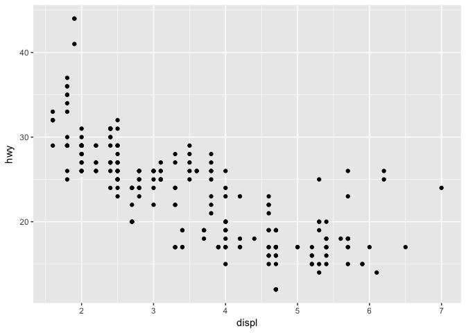
This is the standard plot. Therefore ggplot2 adjust automatically the scales and labels the axis in a nice visual format. We will see later how one can manually modify those graph properties.
You can clearly see a negative correlation. This means that, the bigger the engine the more fuel is needed. But on the far right you can notice a few points lying a bit above the trend. What could those cars be? Hybrids? To answer that question we have to look at the type or class of the car. So let’s continue and add another visual property to our plot.
Aesthetics
As I described earlier ggplot2 uses aesthetic mappings to map the value of variables to a visual property like position of x and y axis on the grid. But you can also map to a color (or british english: colour), shape or size (see bottom for a list of aesthetics) which adds somehow a 3rd dimension. So let us now extend our aesthetics in the plot with aes(x = displ, y = hwy, color = class).
ggplot(data = mpg) +
  geom_point(mapping = aes(x = displ, y = hwy, color = class))

Now we can see what observations belong to which type of car. So our hybrid cars are actually two seaters, smaller or lighter cars which need less fuel. The big SUV and Pickup cars are as suspected on the lower edge.
Again ggplot2 chooses automatically an appropriate color scheme. Try out the two other aesthetics (shape and size) by yourself. Notice that for color and shape it makes sense to map them to a categorical variable where as size is appropriate for continuous variables. The shape aesthetic has also a maximum of 6 values. But if your data should have more than 6 levels, you must specify them manually (R has 25 built in shapes that are identified by numbers).
You can also use logical expression for an aesthetic like color. Try e.g. aes(x = displ, y = hwy, color = displ > 5). This will seperate your data in red and blue observations based on the logical expression.
List of aesthetics:
- x (required)
- y (required)
- alpha
- colour
- fill
- group
- shape
- size
- stroke
For further information about aesthetics take a look at the cran specification.
Facets
Let us now learn more about a cool feature of ggplot2 which suits perfectly to look at categorical variables, the facets. Facets are basically subplots within a plot. So for each level of a categorical variable you get a plot.
Therefore you need to add the facet_wrap() function to your plot and specify by a formula object (name of a data structure in R, not a synonym for equation. Formulas use the tilt sign ~. They can also be used to build models). The formula defines on which variable the subplots are created.
ggplot(data = mpg) +
  geom_point(mapping = aes(x = displ, y = hwy)) +
  facet_wrap(~ class)

As always ggplot2 automatically aligns the subplots. But you can also specify the number of rows or columns, e.g. facet_wrap(~ class, nrow = 2).
The use of formula expression along with facet_grid() allows you to combine two variables. Let us look on all subplots of combinations of drive type (drv) and cylinders (cyl)
ggplot(data = mpg) +
  geom_point(mapping = aes(x = displ, y = hwy)) +
  facet_grid(drv ~ cyl)

Geometric Objects
You can use different visual objects to represent data. Till now we used points as a geometrical object to create a scatterplot. In ggplot2 such objects are called geom. There are different types of geoms. Here is an excerpt of the most important:
geom_point()- plot a scatterplotgeom_line()- plot a line graphgeom_smooth- plot a smooth line fitted to the datageom_bar()- plots bars like a histogramgeom_density()- plots a density graph for continuous datageom_boxplot()- plots a boxplot
All in all over 30 geoms are provided and extension packages provide even more (see https://www.ggplot2-exts.org for a sampling). Similarily, look at the ggplot2 reference or check out the cheatsheet for further information.
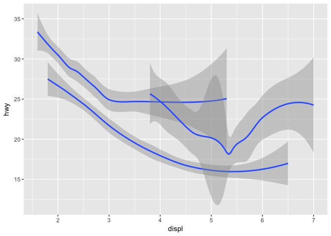
Let’s have a look how differently our scatterplot is represented as a smoothed line plot.
ggplot(data = mpg) +
  geom_smooth(mapping = aes(x = displ, y = hwy))

Here you clearly see the upspike at the end which again is due to our two seater cars.
Note that each geom in ggplot2 takes a mapping argument. However, not every aesthetic works with every geom. The shape aaesthetic makes sense for a point geom, but for a line geom. On the other hand, you can set the linetype of a line, not of a point.
So let us plot different line styles for each drive type (drv 4 = four-wheel drive, f = front-wheel drive and r = rear-wheel drive):
ggplot(data = mpg) +
  geom_smooth(mapping = aes(x = displ, y = hwy, linetype = drv))

As you maybe notice, the lines do not all go from begining till end. This is due to the fact that there is not enough data for this combinations.
Another way to distinguish the line plot between the drivetrain types (drv) would be to use the color aesthetic again. But there is also the so called group aesthetic which groups the data according to the factor levels. The difference lies in the coloring scheme. There is also no legend provided with group.
ggplot(data = mpg) +
  geom_smooth(mapping = aes(x = displ, y = hwy, group = drv))
Try out the color aesthetic yourself to see the difference
Multiple geoms
Now it is time to enrich our plot even further and use multiple geoms. How about combining geom_point() with geom_smooth:
ggplot(data = mpg) +
  geom_point(mapping = aes(x = displ, y = hwy)) +
  geom_smooth(mapping = aes(x = displ, y = hwy))

As explained earlier, the structure of ggplot2 is to add graphical elements to your base function (empty plot: ggplot()). Here we simply add the two geoms to the plot. You might ask yourself, but what if i want to change the aesthetics, then i have to change them in both geom objects. You are right, and this duplication can be avoided by defining the mappings already in the base function of ggplot(). So we will treat these mappings as global mappings that apply to each geom in the graph. Hence,
ggplot(data = mpg, mapping = aes(x = displ, y = hwy)) +
  geom_point() +
  geom_smooth()
will create the same plot. If you add now mappings into the geom objects, they will be treated as local mappings. They extend or overwrite the global mappings for that layer only.
You can go even further and define new data for a layer in the geom object: geom_smooth(data = filter(mpg, class == "subcompact"))
Note:
filter()is a function of thedplyrpackage.
ggplot(data = mpg, mapping = aes(x = displ, y = hwy)) +
  geom_point(mapping = aes(color = class)) +
  geom_smooth(data = filter(mpg, class == "subcompact"), se = FALSE)

Statistical charts
One of the plots which can give a nice and easy overview about the frequency of variables are bar charts. In ggplot2 we can use geom_bar(). To go further into the details of the functionality we will use the diamonds data set contained in the ggplot2 package. There are about 54,000 diamonds, including the price, carat, color, clarity, and cut of each diamond.
ggplot(data = diamonds) +
  geom_bar(mapping = aes(x = cut))
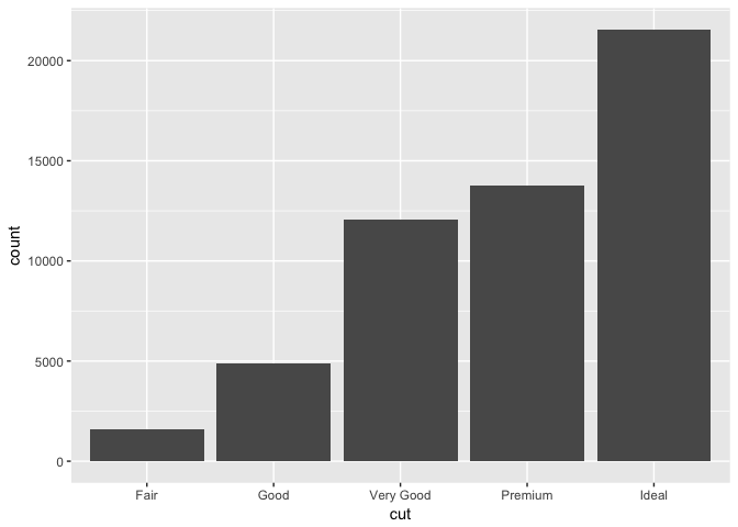
You can see that there are a lot more diamonds with great cut quality than with bad quality. You may notice that this time, there is now y aesthetic mapped to a variable. Despite, there is a count variable as y axis. This variable is automatically generated by ggplot2. New values are also calculated by other plots like e.g. histograms and frequency polygons bin your data and then plot bin counts. Or the already seen smooth geom object fit a model to your data and then plots the predictions.
The method behind that generation of new values is stat. This leads us to the notion of statistical transformation. For geom_bar() the default stat argument is count (see ?geom_bar). So it uses the stat_count() method. Vice versa, ever stat method has also by default a geom object. Hence,
ggplot(data = diamonds) +
  stat_count(mapping = aes(x = cut))
would generate the same bar chart. But sometimes it is nicer to see the proportions rather than the absulute counts. Therefore, we can specify the y aesthetic with ..prop... This overrides the default mapping from transformed variables to aesthetics.
ggplot(data = diamonds) +
  geom_bar(mapping = aes(x = cut, y = ..prop.., group = 1))

In ggplot2 you have over 20 stat functions (see ?stat_bin or the cheatsheet).
Another example would be to use stat_summary(). We will specify some of its parameters to mimic a boxplot with min, max and median values of the total depth of the diamonds (y axis) grouped by their cut quality (x axis).
ggplot(data = diamonds) +
  stat_summary(
    mapping = aes(x = cut, y = depth),
    fun.ymin = min,
    fun.ymax = max,
    fun.y = median
  )

Now let’s bring some color into the game. We already know that we can use the color aesthetic to map a color for points or lines to a variable. This is also possible for bar geom objects. Just set the same varible of the x aesthetic to the color aesthetic, e.g. aes(x = cut, color = cut). But this will give the bars a colored frame and will not fill them with colors. Try your own…
For bar charts it is better to use fill aesthetic. So it is even possible to visualize more variables. Let us look at the different distribution of the clarity(I1 = worst, …, IF = best) meassures within each cut quality:
ggplot(data = diamonds) +
  geom_bar(mapping = aes(x = cut, fill = clarity))
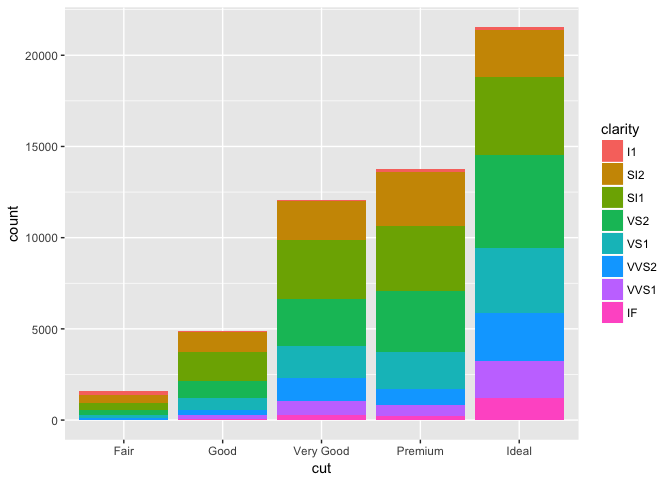
We see that the best quality diamonds, also have the most clear diamonds. Such bar charts are called stacked bar charts. This leads us again to another notion of position adjustment which is specified by the position argument in the bar_geom() (like the stat argument). By default the position parameter is set to "stack". Hence,
ggplot(data = diamonds) +
  geom_bar(mapping = aes(x = cut, fill = clarity), position = "stack")
would produce the same stacked bar chart. But there are also other position adjustments like e.g. position = "fill" or position = "dodge". Try them out yourself.
ggplot(data = diamonds) +
  geom_bar(mapping = aes(x = cut, fill = clarity), position = "dodge")

Coordinate functions
Almost done… Now we will cover coordinate functions to complement the structural template of building plots with ggplot2. By default the Cartesian coordinate system is used. The x and y positions determine the location of the points on the plot. There are several other coordinate systems that helpful for different use cases.
With coord_flip() you are able to change the x and y axis. This can be useful if the labels on the x axis of your original plot are too big. Look at this boxplot. If the axis where flipped the labels would be impossible to read.
ggplot(data = mpg, mapping = aes(x = class, y = hwy)) +
  geom_boxplot() +
  coord_flip()

Template and Structure of ggplot
Below in the code snippet you can see the general template for building plots in ggplot2. The values in brackets (<...>) are variables which the user has to define. Not all are needed to be specified, ggplot2 provides useful default values; except for the data, geoms, and mappings.
ggplot(data = <DATA>) +
  <GEOM_FUNCTION>(
     mapping = aes(<MAPPINGS>),
     stat = <STAT>,
     position = <POSITION>
  ) +
  <COORDINATE_FUNCTION> +
  <FACET_FUNCTION>
If you follow this formal system, you can describe any plot as a combination of a dataset, a geom, a set of mappings, a stat, a position adjustment, a coordinate system, and a faceting scheme.
I hope the examples could give you a basic understanding about the structure of ggplot2. In further blog posts we will go more in depth on how to custumize plots and we will look at specific plot types.